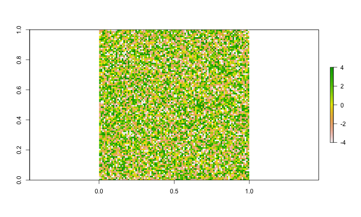
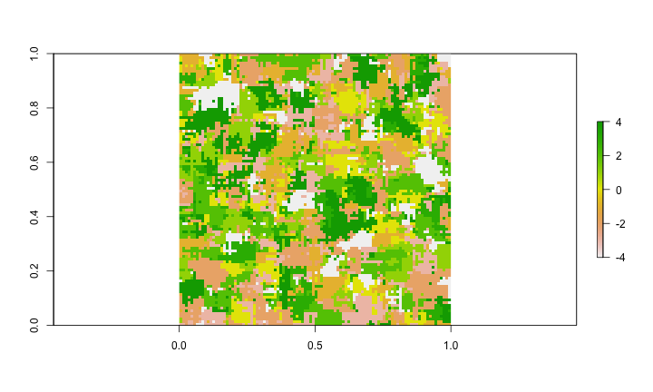
Kernels for everyone!
During my dissertation, I spent a lot of time working on spatial kernel estimates. Where spatial kernel estimates are defined as a convolution of a spatial suppport ,
The kernelDensityEstimates package provides a means to apply these estimates to raster S4 objects from the NA values, and uses OpenMP for acceleration.
However, all processing is done in memory, so there is no support for extremely large images.
The rasterKernelEstimates R package is currently not on CRAN, but will be after the documentation is cleaned up. Furthermore, the implementation of the kernels is currently non-optimal, and a fair bit of work can be done to speed them up a bit more. For those interested in helping out, the code is on my github page.
A short example of each function is provided below with some basic performance metrics. All timings are done on a Late 2013 MacBook Pro 13" with a dual-core 2.4Ghz i5 running R 3.3.1 compiled under gcc 6.1.0.
rasterLocalSums
The function rasterLocalSums calculates a weighted sum of pixel values in a spatial neighborhood defined by the matrix W,
focal when fun is not specified.
In fact, the results are identical when padding is used in the focal call.
library(raster)
library(rasterKernelEstimates)

set.seed(100)
n <- 500

# create a raster object
r <- raster::raster( matrix(rnorm(n^2),n,n))

# create a weight matrix
W <- raster::focalWeight(r,c(1,0.04),type='Gauss')

# apply the weight with rasterKernelEstimates
run.time <- proc.time()
rLocalKDE1 <- rasterLocalSums(r,W)
print(proc.time() - run.time)
##    user  system elapsed
##   0.975   0.004   0.325
# apply the weight with the raster packages focal
run.time <- proc.time()
rLocalKDE2 <- raster::focal(r,W,pad=TRUE)
print(proc.time() - run.time)
##    user  system elapsed
##   0.667   0.008   0.678
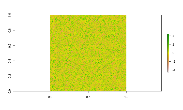
# plot original image
plot(r)
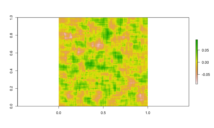
# plot the smoothed image
plot(rLocalKDE1)
# print out the max abs difference
print(
sprintf(
  "The maximum absolute difference = %f.",
    max(abs(values(rLocalKDE1) - values(rLocalKDE2)
    ),na.rm = T))
)
## [1] "The maximum absolute difference = 0.000000."
rasterLocalQuantiles
The function rasterLocalQuantiles calculates the quantile of pixel values in a spatial neighborhood defined by the matrix W;
This result should generally be reproducible using the raster library function focal when fun is specified as quantile.
Because quantiles do not necessarily fall exactly on order statistics there is a need to map quantiles between a function of the order statistics.
In the rasterLocalQuantiles function this mapping is done to the closest odd-valued-index order statistic.
E.g. if the quantile falls between the first and second order statistic.
This approach matches the inverse empirical cdf transform used by the type=1 transform in the stats::quantile function.
Note that the quantile function applied to raster objects calculates the quantile from all pixels, not local quantiles.
As far as applications go, this function is particularly useful when working with data with a large number of outliers.
library(raster)
library(rasterKernelEstimates)


set.seed(100)
n <- 100

# create a raster object with extreme values
r <- raster::raster( matrix(rcauchy(n^2),n,n))

# create a weight matrix
W <- matrix(1,nrow=3,ncol=3)

# calculate local median
run.time <- proc.time()
rLocalKDE1 <- rasterLocalQuantiles(r,W,q=30)
print(proc.time() - run.time)
##    user  system elapsed
##   0.018   0.001   0.010
# calculate local median
run.time <- proc.time()
rLocalKDE2 <- raster::focal(
  r, W, pad=TRUE,
  fun=function(x) stats::quantile(x,probs=0.3,na.rm=T,type=1),
  padValue=NA)
print(proc.time() - run.time)
##    user  system elapsed
##   1.245   0.010   1.268
# plot boxplot of original image
boxplot(r)
# plot the smoothed image
plot(rLocalKDE1)
# print out the max abs difference
print(
sprintf(
  "The maximum absolute difference = %f.",
    max(abs(values(rLocalKDE1) - values(rLocalKDE2)
    ),na.rm = T))
)
## [1] "The maximum absolute difference = 0.000000."
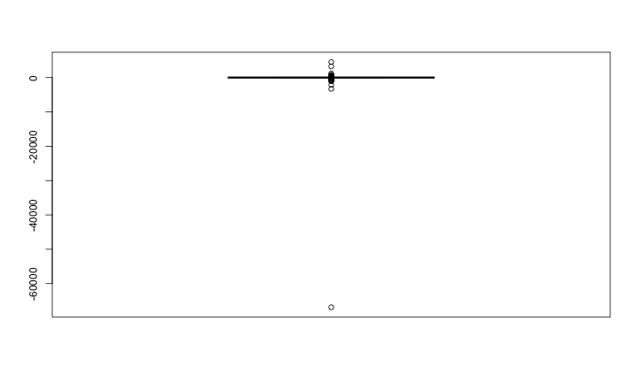
r.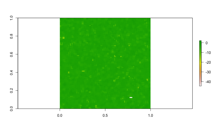
rasterLocalMoments
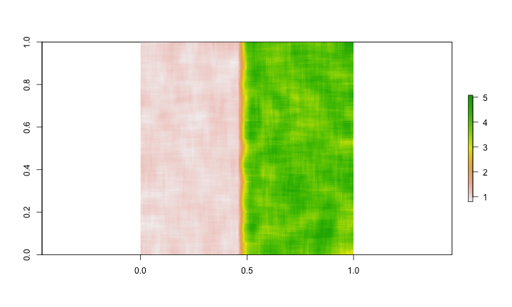
The function rasterLocalMoments calculates up to the second moment over the weighted matricies Wmu and Wvar,
rasterLocalSums is the normalization of the weights. This ensures the weights sum to one.
library(raster)
library(rasterKernelEstimates)

set.seed(100)
n <- 200

# create a raster object of two populations
r <- raster::raster(
  cbind( matrix(rnorm(n^2),n,n), matrix(rnorm(n^2,2,2),n,n)) )


# create a weight matrix
W <- raster::focalWeight(r,c(1,0.04),type='Gauss')

# calculate the weighted local mean and variance
run.time <- proc.time()
rLocalKDE1 <- rasterLocalMoments(r,W)
print(proc.time() - run.time)
##    user  system elapsed
##   0.343   0.002   0.102
# plot original image
plot(r)
# plot the weighted mean
plot(rLocalKDE1$mu)
# plot the weighted variance
plot(rLocalKDE1$var)
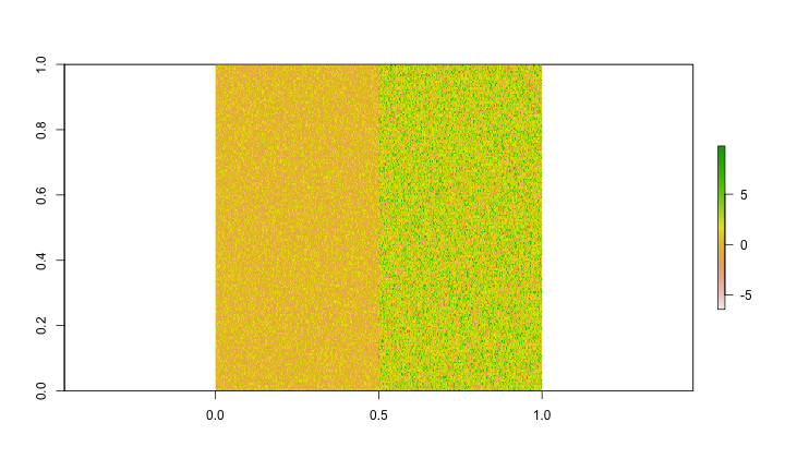
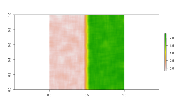
rasterLocalCategorical Modes
The function rasterLocalCategoricalModes calculates a categorical mode from a raster image over the weighted spatial neighborhood devined by the matrix W,
r.
library(raster)
library(rasterKernelEstimates)

set.seed(100)
n <- 100

# create a categorical raster
r <- raster::raster(
  matrix( sample(-4:4,size=n^2,replace=T),n,n)
  )


# create a weight matrix
W <- matrix(1,9,9)

# calculate the weighted local mean and variance
run.time <- proc.time()
rLocalKDE1 <- rasterLocalCategoricalModes(r,W)
print(proc.time() - run.time)
##    user  system elapsed
##   0.030   0.000   0.011
# plot original image
plot(r)
# plot the weighted mean
plot(rLocalKDE1)
