meanShiftR
In this blog post, I will be introducing the meanShiftR package. meanShiftR is a rewrite of my original mean shift R package from 2013, based on the Fast Library for Approximate Nearest Neighbors (FLANN). The meanShiftR package is focused on providing to R users the most computationally efficient mean shift implementations available in the literature. This includes approximations to the mean shift algorithm through kernel truncations and approximate nearest-neighbor (ANN) approaches.
The mean shift algorithm is a steepest ascent classification algorithm, where classification is performed by fixed point iteration to a local maxima of a kernel density estimate. This method is originally credited to (Fukunaga and Hostetler, 1975), but didn't see wide-scale adoption until it was popularized by (Cheng, 1995). This algorithm has a fairly simple form of a convex combination of the support of the kernel density estimate, where the weight is calculated from the function , the derivative of kernel . In the computer science literature this function is commonly refered to as the profile and is refered to as the shadow kernel.
The explicit formulation of the mean shift for (the point being classified) is,
This algorithm identifies local maxima by updating at each iteration, starting with a set of initial points. Iteration continues until a fixed number of iterations is met or where is an acceptable tolerance.
R Implementations
On CRAN there are two other packages that perform the mean shift algorithm, MeanShift and LPCM. The MeanShift package provides multi-core acceleration, a large number of kernels, and support for blured mean shift. LPCM provides a fast and effective mean shift implementation, as well as plotting and diagnostic tools. LPCM is restricted to just Gaussian kernels and does not provide any multi-core acceleration.
The meanShiftR package presented here is considerably faster than the prior two packages, but currently lacks diagnostic tools and support for more kernels. Instead, the meanShiftR package provides a number of ways to speed mean shift. This includes a generalized Gaussian variant of the mean shift (Lisic, 2015) providing accelerated convergence at the expense of some numerical stability, and support for support truncation with nearest neighbor and approximate nearest neighbor searches. Furthermore, this mean shift implementaiton allows for mean shifting on a separate data set than the kernel support, a feature missing in the other two packages.
A quick speed comparison was done between the three packages, this was performed on a 13" MacBook Pro with a dual-core hyper-threaded CPU. In this configuration the default number of cores used by MeanShiftR is four. A slight change had to be done to the MeanShift package to provide similar results, mainly the terminal condition had to be modified to be equivalent to meanShiftR and LPCM. This terminal condition is simply the relative L distance.
library(meanShiftR)
library(LPCM)
library(MeanShift)

# set a seed to make this reproducible
set.seed(100)

# set the number of iterations to test
# (we will terminate well before this)
iter <- 1000

# set the number of points to simulate
n <- 500

# set the bandwidth
h <- c(0.5,0.5)

# create example data
x1 <- matrix( rnorm( n ),ncol=2)
x2 <- matrix( rnorm( n ),ncol=2) + 2
x <- rbind( x1, x2 )

#plot initial points
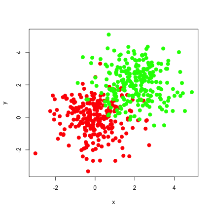
plot(x, col=rep(c('red','green'),each=n/2),
     cex=2, xlab='x',ylab='y',pch=20)
########### meanShiftR ###################
run.time <- proc.time()
result <- meanShift(
  x,
  x,
  algorithm="KDTREE",
  bandwidth=h,
  alpha=0,
  iterations = iter,
  parameters=c(10,100)
)
meanShiftR_kd_runtime <- (proc.time()-run.time)[3]

# assignment
meanShiftR_kd_assignment <- result$assignment

# value
meanShiftR_kd_value <- result$value


########### meanShiftR ###################
run.time <- proc.time()
result <- meanShift(
  x,
  x,
  bandwidth=h,
  alpha=0,
  iterations = iter
)
meanShiftR_runtime <- (proc.time()-run.time)[3]

# assignment
meanShiftR_assignment <- result$assignment

# value
meanShiftR_value <- result$value


########### LPCM ###################
runtime <- proc.time()
result <- ms(
            x,
            h=h,
            scaled=FALSE,
            iter=iter,
            plotms=-1)
LPCM_runtime <- (proc.time()-runtime)[3]

# assignment
LPCM_assignment <- result$cluster.label

# value
LPCM_value <- result$cluster.center[LPCM_assignment,]


########### MeanShift ###################
options(mc.cores = 4)
z <- t(x)
runtime <- proc.time()
result <- msClustering(
            X=z,
            h=h,
            kernel="gaussianKernel",
            tol.stop=1e-08,
            tol.epsilon=1e-04,
            multi.core=T)
MeanShift_runtime <- (proc.time()-runtime)[3]

MeanShift_assignment <- result$labels
MeanShift_value <- t(result$components[,result$labels])

# print
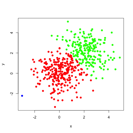
plot(x, col=sapply(meanShiftR_assignment,function(x)c('red','green','blue')[x]),
   cex=1.5, xlab='x',ylab='y',pch=20)
result <- data.frame(
  runtime=c( meanShiftR_runtime,
                meanShiftR_kd_runtime,
                LPCM_runtime,
                MeanShift_runtime),
  maxDiff=c(max(abs(meanShiftR_value - LPCM_value)),
               max(abs(meanShiftR_kd_value - LPCM_value)),
               0,
               max(abs(MeanShift_value - LPCM_value))
               ),
  assignmentDiff=c(sum(meanShiftR_assignment != LPCM_assignment),
               sum(meanShiftR_kd_assignment != LPCM_assignment),
               0,
               sum(MeanShift_assignment != LPCM_assignment)
               )
  )

colnames(result) <- c('Run-Time',
                      'Maximum Absolute Difference',
                      'Label Disagreements')

rownames(result) <- c('meanShiftR',
                      'meanShiftR K-D Tree',
                      'LPCM ms',
                      'meanShift msClustering')

library(xtable)
print(xtable(result,digits=6,display=c('s','f','f','d')), type='html')
| Run-Time | Maximum Absolute Difference | Label Disagreements | |
|---|---|---|---|
| meanShiftR | 0.304000 | 0.000000 | 0 |
| meanShiftR K-D Tree | 4.871000 | 0.000000 | 0 |
| LPCM ms | 2.425000 | 0.000000 | 0 |
| meanShift msClustering | 43.168000 | 0.000000 | 0 |


Here we can see some pretty good performance results for meanShiftR relative to the other R packages. Unfortunately the k-d tree based implementation wasn't as fast as I would have liked, but its utility is really in tuncated support kernels. Support for these kernels will be added later.
It is unclear why the performance of MeanShift was so poor relative to the other approaches. To verify that it was not a function of the parallel implementation, the algorithm was run with one thread achieving approximately 50% of the performance with mc.cores=4.
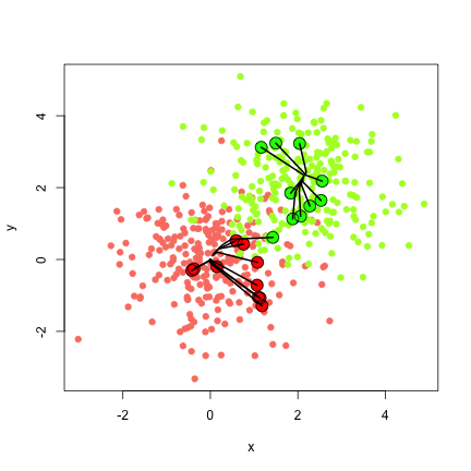
Diagnostic plots are not yet included, but convergence path plots can be easily generated by looping over single iterations. An example is provided below, with results in Figure 3.
library(meanShiftR)
library(LPCM)
library(MeanShift)

# set a seed to make this reproducible
set.seed(100)

# set the number of iterations to test
# (we will terminate well before this)
iter <- 10

# set the number of points to simulate
n <- 500
m <- 20

# set the bandwidth
h <- c(0.5,0.5)

# create example data
x1 <- matrix( rnorm( n ),ncol=2)
x2 <- matrix( rnorm( n ),ncol=2) + 2
x <- rbind( x1, x2 )

# create some test data for diagnostic plots
y1 <- matrix( rnorm( m ) ,ncol=2)
y2 <- matrix( rnorm( m ),ncol=2) + 2
y <- rbind( y1, y2 )

plot(x, col=rep(c('salmon','greenyellow'),each=n/2),
   cex=1.5, xlab='x',ylab='y',pch=20)

points(y,col=rep(c('red','green'),each=m/2),
       cex=2,pch=19)

points(y,cex=2)

########### meanShiftR ###################

#initial run
result <- meanShift(
    y,
    x,
    algorithm="KDTREE",
    bandwidth=h,
    alpha=0,
    iterations = iter,
    parameters=c(10,100)
)

y0 <- rbind(y,result$value)

for( i in 2:iter) {

  result <- meanShift(
    result$value,
    x,
    algorithm="KDTREE",
    bandwidth=h,
    alpha=0,
    iterations = 1,
    parameters=c(10,100)
  )

  # concate on the result
  y0 <- rbind(y0,result$value)
}

# plot the paths

for( i in 1:m ) {
  pointIndex <- seq(from=0,to=(m*(iter-1)),by=m)+i
  points(y0[pointIndex,] , type='l',lwd=2)
}

Future Plans
Due to issues with stack size limits in .C, I was unable to directly submit the original FLANN based package to CRAN, therefore a complete rewrite in C has been initiated. This 0.50 release, is the first release on-the-way to 1.00, where feature parity will be met with the original code.
The release map for this package follows four more planned releases:
- 0.50 - Initial release.
- 0.60 - Distance-based k-d trees, and support for popular kernels.
- 0.70 - Dual-tree acceleration (Wang et al., 2007).
- 0.80 - Fast Guassian Transform acceleration (Xia et. al. 2010).
- 0.90 - Merge-Tree acceleration (Lisic, 2015).
- 1.00 - Smoothing the support and diagnostic tools.
References
Cheng, Y. (1995). Mean shift, mode seeking, and clustering. IEEE transactions on pattern analysis and machine intelligence, 17(8), 790-799.
Fukunaga, K., & Hostetler, L. (1975). The estimation of the gradient of a density function, with applications in pattern recognition. IEEE Transactions on information theory, 21(1), 32-40.
Lisic, J. (2015). Parcel Level Agricultural Land Cover Prediction (Doctoral dissertation, George Mason University).
Wang, P., Lee, D., Gray, A. G., & Rehg, J. M. (2007, March). Fast Mean Shift with Accurate and Stable Convergence. In AISTATS (pp. 604-611).
Xiao, C., & Liu, M. (2010, September). Efficient Mean‐shift Clustering Using Gaussian KD‐Tree. In Computer Graphics Forum (Vol. 29, No. 7, pp. 2065-2073). Blackwell Publishing Ltd.


