The cdlTools R package
This is a brief tutorial on the cdlTools package developed by Lu Chen and I to download and perform some simple analysis on USDA's cropland data layer (CDL). This tutorial will cover downloading CDL data, obtaining some zonal statistics, and explore land cover change. This package is not currently available on CRAN, but is available via github, and can be installed through Hadley Wickham's devtools package.
The cropland data layer is a set of raster images classified into up-to 256 possible land uses across the coterminous 48 states in the United States. The temporal coverage extends from 2008 to present, with some states having earlier coverage. Details on the classification process can be found in (Boryan et al, 2011). This tutorial will be broken into three parts:
Downloading CDL raster images
CDL raster data can be downloaded directly through the CDL website. However, it is not always convenient to manually download the data and extract it to a directory. This task can be easily accomplished through the cdlTools package.
To do this we first need to load the cdlTools package. Hadley Wickham's devtools works well for this job.
library(devtools)
install_github('jlisic/cdlTools')
library(cdlTools)
In the next step we want to download the CDL raster images in geotiff format to a local directory from USDA's cropscape server. The directory I'm saving these raster images to is the CDL directory in my home folder. It is important to make sure that this directory exists first. Note, that the CDL cache may not be populated for 2015, so if this example doesn't work you may want to change the year range to 2008:2014. It's also possible to just manually download the files below through the cropscape web interface and extract them to a directory.
# years to query
years <- 2008:2015
state <- 'maryland'

cdl.raster <- getCDL(state,years,location="~/CDL")
If you already have the data in CDL_YYYY_FF.tif form, where YYYY is the year and FF is the two digit fips code, you can just use a file url to define the directory. Note: This may or maynot work depending on your operating system and method for download.file.
cdl.raster <- getCDL(state,years,alternativeUrl="file:///Users/jonathanlisic/CDL")
If you want to be fancy and setup an anonymous FTP of HTTP server, you can just download the data to that server. Then, access it through the alternativeUrl parameter. This is useful for organizations that may want to conserve bandwidth or improve performance of applications in a network.
cdl.raster <- getCDL(state,years,alternativeUrl="ftp://10.0.1.1/CDL/CDL_Maryland")
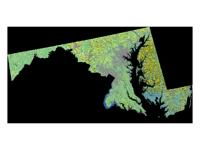
Once you have downloaded the data you can plot the results.
library(raster)
plot(cdl.raster$`2015`)

Zonal statistics
The gdalUtils package provides several functions offered by the GDAL library. This includes rasterization of vector files. Rasterization of vector files is an effective way to quickly calculate statistics for areal units within a CDL raster image.
In this example we are going to quickly calculate corn pixels per county in Maryland. To do this we are first going to use the gdal function gdal_rasterize. It is assumed that this command is in the path of the system it is run on. An alternative is to use the gdalUtils package, but I wrote this function and most of cdlTools before this package existed and haven't had time to modify rasterExtract. To get the county boundaries we are also going to download some U.S. census county data for 2010.
# rasterExtract is a quick function that polygonizes a SpatialPolygonsDataFrame 'x'
# to a given raster image extent and resolution 'r' with values specified
# by 'variable' in
rasterExtract <- function(x,r,variable) {

  tempTif <- tempfile(fileext=".tif")
  tempShp <- tempfile(fileext=".shp")

  # write polygon
  writeOGR(x,dirname(tempShp),gsub("[.]shp","", basename(tempShp)),driver="ESRI Shapefile",overwrite=TRUE)

  # use gdalPolygonize
  if( missing(variable) ) {
    system(
        sprintf( "gdal_rasterize  -burn 1 -ot UInt32 -a_nodata 0 -a_srs '%s' -tr %f %f -te %f %f %f %f %s %s",
                  projection(r), xres(r), yres(r), xmin(r), ymin(r), xmax(r), ymax(r),
                  tempShp, tempTif)
         )
  } else {
    system(
        sprintf( "gdal_rasterize  -a '%s' -ot UInt32 -a_nodata 0 -a_srs '%s' -tr %f %f -te %f %f %f %f %s %s",
                  variable, projection(r), xres(r), yres(r), xmin(r), ymin(r), xmax(r), ymax(r),
                  tempShp, tempTif)
         )
  }

  # create a new raster object
  r.out <- raster(extent(r), ncols=ncol(r), nrows=nrow(r), crs=projection(r))
  values(r.out) <- values(raster(tempTif))

  # free up the data
  unlink(tempTif)
  unlink(tempShp)

  return(r.out)
}

library(rgdal)
library(rgeos)

# download shape files
url <- sprintf("https://www2.census.gov/geo/tiger/TIGER2010/COUNTY/2010/tl_2010_%02d_county10.zip",fips(state))
download.file(url,destfile=sprintf('~/CDL/tl_2010_%02d_county10.zip',fips(state)))

#unzip
unzip(sprintf('~/CDL/tl_2010_%02d_county10.zip',fips(state)),exdir='~/CDL')

#load
county <- readOGR(path.expand('~/CDL'),sprintf('tl_2010_%02d_county10',fips(state)))
## OGR data source with driver: ESRI Shapefile
## Source: "/Users/jonathanlisic/CDL", layer: "tl_2010_24_county10"
## with 24 features
## It has 17 fields
#re-project
county <- spTransform(county,projCDL)

#rasterize the shape files for maryland counties
county.raster <- rasterExtract(county, cdl.raster$`2015`,'COUNTYFP10')

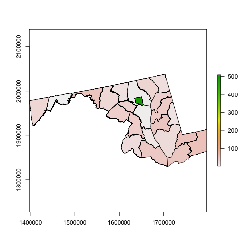
#plot out our current output to check if things look sane
plot(county.raster)
plot(county,add=T)

Finally, we are going to calculate the zonal statistics with the matchCount function in cdlTools. This function takes two raster images and calculates the number of pairs in each image.
library(dplyr)
# we use matchCount to get the matched pairs between the rasters
# the parameter m is set to the maximum value in either raster image
cropByCounty <- matchCount(county.raster,cdl.raster$`2015`,m=510)
cropByCounty <- as.data.frame(cropByCounty)

# get all CDL classes that contain corn, available in the cdlTools 'corn' data
cornByCounty <- subset(cropByCounty,CDL_2015_24 %in% corn)

tmp <- county@data
tmp$layer <- as.numeric(as.character(county@data$COUNTYFP10))
cornByCounty <- left_join(cornByCounty, tmp, by=c("layer"="layer"))
aggregate(count ~ NAME10, data=cornByCounty,sum)
##             NAME10  count
## 1         Allegany   4001
## 2     Anne Arundel  18101
## 3        Baltimore  89781
## 4          Calvert  14012
## 5         Caroline 162192
## 6          Carroll 140647
## 7            Cecil 117161
## 8          Charles  21131
## 9       Dorchester 109068
## 10       Frederick 166194
## 11         Garrett  21036
## 12         Harford 100710
## 13          Howard  28593
## 14            Kent 191487
## 15      Montgomery  40234
## 16 Prince George's  12844
## 17    Queen Anne's 221128
## 18        Somerset  58131
## 19      St. Mary's  34430
## 20          Talbot 123497
## 21      Washington 100252
## 22        Wicomico 104576
## 23       Worcester 154048
Land cover change
Year-to-year land cover change is now available through the cropscape. However, the API documentation does not say how to query this new data, nor is it possible to extend to longer lags, e.g. corn-soybeans-corn.
To calculate year-to-year change you first need to have raster images that match. This can be a bit of a problem with the CDL data since some earlier years are at 56 by 56 meters, instead of the current 30 by 30 meters. To get everything to match, we will use the resample function from the raster package. Note, that this function can take quite a while to run.
# Figure out what needs to be resampled to match our latest year's projection and extent.
cdl.raster.resample <- sapply(
  cdl.raster,
  function(x) !identical( extent(x), extent(cdl.raster[[as.character(last(years))]]) )
  )

# Resample the data, this may take a while.  It is possible to accelerate this operation
# with the snow package.
cdl.raster.resampled <- lapply(
  cdl.raster[ cdl.raster.resample ],
  function(x) resample( x, cdl.raster[[as.character(last(years))]],method="ngb" )
  )
cdl.raster[ cdl.raster.resample ] <- cdl.raster.resampled

# Create raster brick, this also is pretty slow.
cdl.brick <- brick(cdl.raster)
After resampling, we went ahead and put all the images into a raster brick. We will now use this brick to get the year to year change of all crops. Because, all these operations do take a while, the resulting csv is provided and can be downloaded here.
# Get year-by-year change in tidy format.
a <- subset(cdl.brick,sprintf('X%d',first(years)))
result <- c()
for(year in years[-1]) {
  b <- subset(cdl.brick,sprintf('X%d',year))
  d <- matchCount(a,b,m=256)
  d <- cbind(d,year)
  colnames(d) <- c('In','Out','Pixels','Year')
  d.df <- as.data.frame(d)
  result <- rbind(result,d.df)
}

write.csv(result,"md-change.csv")
If we are just interested in pixels moving from corn to corn each year, we can simply query the result using dplyr and magrittr.
# assuming we are starting from scratch
library(cdlTools)
library(dplyr)
library(magrittr)

# read in data
mdChange <- read.csv("http://meanmean.me/blogs/cdlTools/md-change.csv")

mdChangeCorn <- mdChange %>%
  subset(In %in% corn & Out %in% corn) %>%
  group_by(Year) %>% summarize(total = sum(Pixels))
References
Boryan, Claire, et al. "Monitoring US agriculture: the US department of agriculture, national agricultural statistics service, cropland data layer program." Geocarto International 26.5 (2011): 341-358.


