Mysteriously Slow sample
Hi everyone, I'm at JSM 2018 right now, so feel free to drop by my session or drop by in the halls! Just give me a tweet!
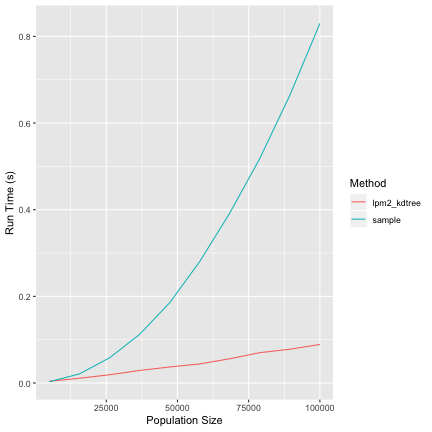
Back to the meat-and-potatoes of this post. A while ago I was running good old sample and comparing its performance to my lpm2_kdtree function in the BalancedSampling package (Grafström and Lisic, 2016).
In this comparison I noticed that sample was in some cases slower than my balanced sampling method when using sampling weights.
library(BalancedSampling)
library(ggplot2)

# sampling proportion
f <- 0.1

# population size
N_values <-  seq(from=5000, to=100000,length=10)

set.seed(99)

pi <- runif(100000)

result <- c()

for( N in N_values) {
  # get sample size
  n <- round(f*N)

  ## run lpm2-kdtree

  start_time <- proc.time()[3]
  # to make things even we normalize pi
  pi_tmp <- pi[1:N] * n/sum(pi)
  # we probably don't want to balance by pi_tmp, but
  # for checking speed this is fine
  lpm2_kdtree(pi_tmp,pi_tmp)
  end_time <- proc.time()[3] - start_time

  result <- rbind(result, c(f, N, 1, end_time ))

  ## run sample

  index <- 1:N

  start_time <- proc.time()[3]
  # to make things even we normalize pi
  sample(index,size=n,prob=pi_tmp)
  end_time <- proc.time()[3] - start_time

  result <- rbind(result, c(f, N, 2, end_time ))
}


colnames(result) <-
  c('SamplingFraction', 'PopulationSize', 'Method','RunTime')
result <- as.data.frame(result)

result[c('SamplingFraction','Method')] <-
  lapply(result[c('SamplingFraction','Method')], as.factor)
levels(result$Method) <- c("lpm2_kdtree","sample")

ggplot( aes(x=PopulationSize, y=RunTime, class=Method), data=result)+
  geom_line(aes(color=Method)) +
  ylab("Run Time (s)") +
  xlab("Population Size")

How could this be?
Let's condsider a few possible reasons.
Are you running an old version of R?
No, this was done with R 3.5.0, but results hold on 3.5.1.
Is this because you are a freedom hating Mac user?
Nope, I get similar results in Linux
Is this due to the revsort in ProbSampleNoReplace found in random.c?
How amazingly prescient of you! If you track down the code path, the method used for sampling has a revsort call right at the begining (Line 323). Some basic testing seems to identify this as the likely culprit. Therefore, it might be possible to speed up sampling by checking if the probabilities are sorted.
Keep in mind that there are likely good reasons for R to use this method relative to others, including the alternative method below. One is computational stability, split sampling through the pivotal methods tends to work well when sample sizes aren't extremely small. However, I don't have any good comparisons of methods, if anyone knows please let me know, doing a literature search on this is pretty far down on my todo list.
That's great, but what can I do to improve my weighted or PPS sampling?
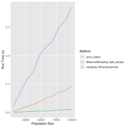
Well, I wrote a quick pivotal method implementation (think LPM2 without balancing) that seems to work. It's available as split_sample on my github version of BalancedSampling.
There is also UPrandompivotal in the sampling package (Tillé and Matei, 2016).
However, my implementation seems to be considerably faster. We will take a look at this in another blog post.
Finally, keep in mind that split_sample probably isn't as well tested as UPrandompivotal. So I'm happy to take any feedback.
library(devtools)
install_github("jlisic/BalancedSampling")
library(BalancedSampling)
library(ggplot2)
library(sampling)

# sampling proportion
f <- 0.1

# population size
N_values <-  seq(from=5000, to=100000,length=10)

set.seed(99)

pi <- runif(100000)

result <- c()

for( N in N_values) {
  # get sample size
  n <- round(f*N)

  ## run lpm2-kdtree

  start_time <- proc.time()[3]
  # to make things even we normalize pi
  pi_tmp <- pi[1:N] * n/sum(pi)
  # we probably don't want to balance by pi_tmp, but
  # for checking speed this is fine
  lpm2_kdtree(pi_tmp,pi_tmp)
  end_time <- proc.time()[3] - start_time

  result <- rbind(result, c(f, N, 1, end_time ))


  ## run pivotal method (BalancedSampling)

  index <- 1:N

  start_time <- proc.time()[3]
  # to make things even we normalize pi
  pi_tmp <- pi[1:N] * n/sum(pi)
  split_sample(pi_tmp)
  end_time <- proc.time()[3] - start_time

  result <- rbind(result, c(f, N, 2, end_time ))


  ## run pivotal sampling (sampling)

  index <- 1:N

  start_time <- proc.time()[3]
  # to make things even we normalize pi
  pi_tmp <- pi[1:N] * n/sum(pi)
  UPrandompivotal(pi_tmp)
  end_time <- proc.time()[3] - start_time

  result <- rbind(result, c(f, N, 3, end_time ))
}


colnames(result) <-
  c('SamplingFraction', 'PopulationSize', 'Method','RunTime')
result <- as.data.frame(result)

result[c('SamplingFraction','Method')] <-
  lapply(result[c('SamplingFraction','Method')], as.factor)
levels(result$Method) <-
  c("lpm2_kdtree","BalancedSampling::split_sample",
    "sampling::UPrandompivotal")

ggplot( aes(x=PopulationSize, y=RunTime, class=Method), data=result)+
  geom_line(aes(color=Method)) +
  ylab("Run Time (s)") +
  xlab("Population Size")

Have a great JSM!
References
Grafström, A., Lisic, J.: BalancedSampling: balanced and spatially balanced sampling. R package version 1.5.2. https://CRAN.R-project.org/package=BalancedSampling. Accessed August 28, 2018. (2016)
Tillé, Y., Matei, M.: sampling: Survey Sampling. R package version 2.8. https://CRAN.R-project.org/package=sampling. Accessed August 28, 2018. (2016)


